Clearly Explaining: Playing Atari with Deep Reinforcement Learning (2013) [1/35]

The Experiment

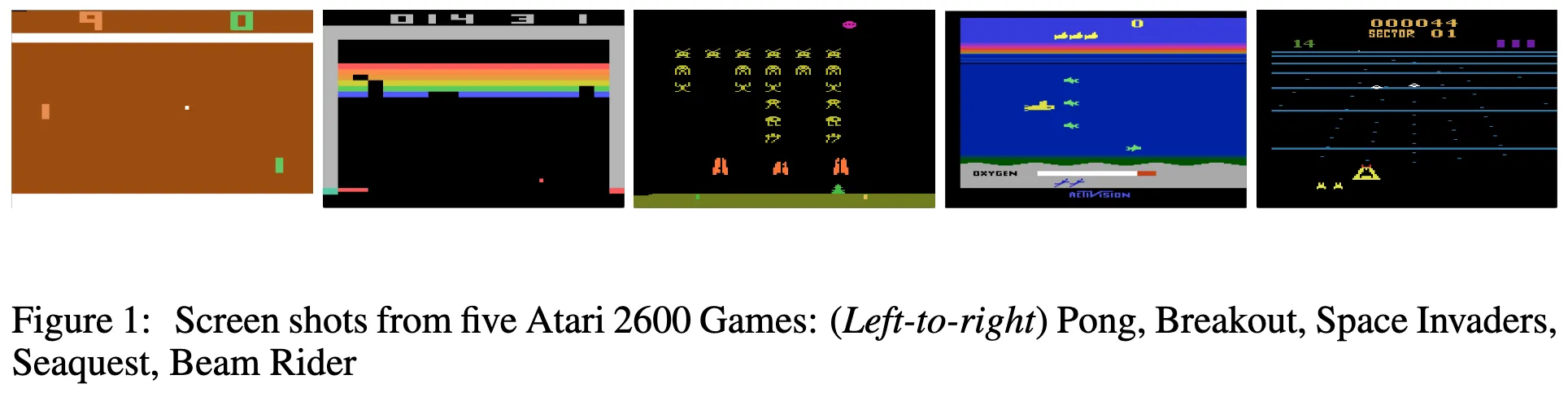
Imagine sitting a computer down in front of an old Atari console. You don’t tell it the rules of Breakout or Space Invaders. You don’t explain what a “paddle” or “ball” is. You just plug in the video cable and the controller, point to the score counter, and say: “Make that number go up.”

In 2013, a small London-based startup called DeepMind ran exactly this experiment. They built an agent and tested it on 7 different Atari 2600 games—with zero game-specific knowledge baked in.

Input: The raw screen pixels (what we see).
Output: Joystick commands (what we do).
Goal: Maximize the game score.

The result? A single neural network architecture learned to master games ranging from Pong to Space Invaders, outperforming all previous methods on 6 out of 7 games and surpassing human experts on 3.

This paper marked the “Big Bang” moment for Deep Reinforcement Learning, laying the groundwork for AlphaGo, robotic control, and modern AI agents.

The seven Atari games used in the experiment

Let’s break down exactly how they did it.

Step 1: Teaching the Agent to “See”

The first challenge was perception. An Atari screen outputs a high-resolution, color image at 60 frames per second. For 2013 hardware, processing this raw feed was too expensive. More importantly, much of that data is irrelevant to game logic. The team made three simplifications:

Grayscale: They removed color, reducing the input to 1 channel. (Color rarely matters for Atari game mechanics).
Downsampling: They shrunk the image to 84 × 84 pixels.
Frame Stacking: A single frame is a snapshot—you can’t tell if the ball is moving up or down. To give the agent a sense of motion, they stacked the last 4 consecutive frames together.

This gave the network a compact but information-rich input: an 84 × 84 × 4 tensor representing the recent visual history of the game.

Step 2: Building the “Brain” (The Network Architecture)

With the input defined, DeepMind needed a model to process these pixels and decide which action to take. They chose a Convolutional Neural Network (CNN), a type of architecture specifically designed for image data.

The network’s job was to transform raw pixels into a single decision: “Which button should I press?”

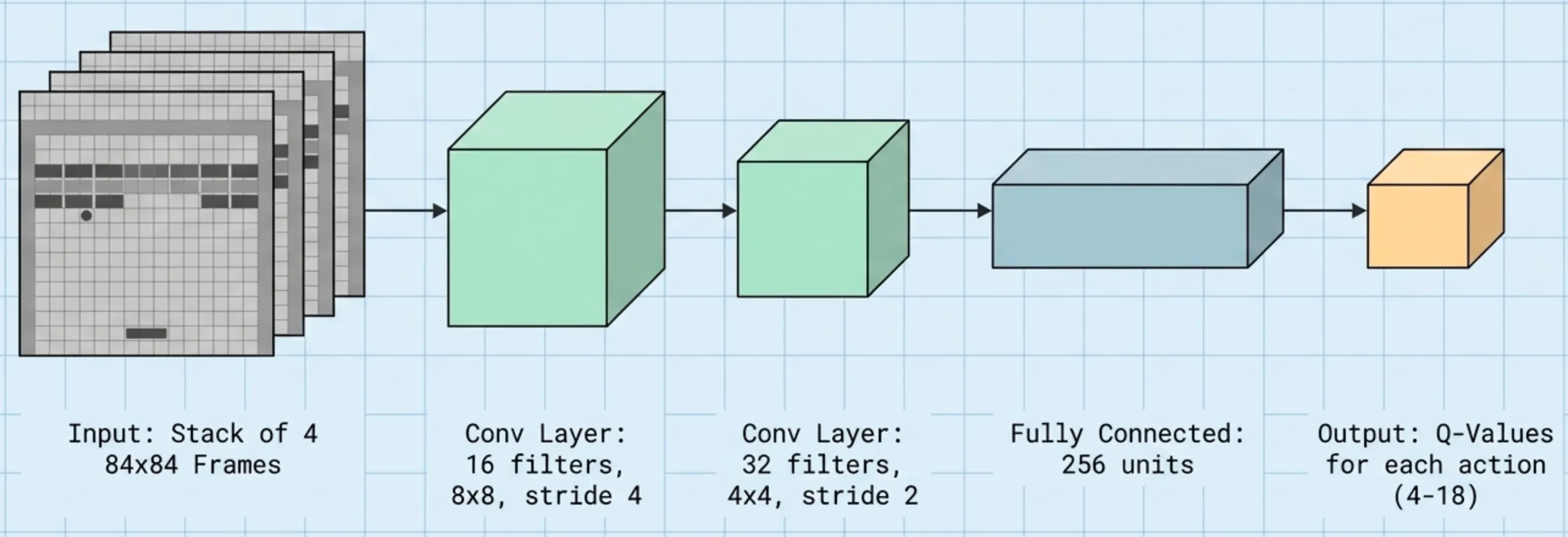
The architecture of the Deep Q-Network

The architecture had three main parts:

Convolutional Layers: These act as pattern detectors. The first layer learns to recognize simple features like edges and corners. The second layer combines those into more complex patterns—shapes that might represent a paddle, a ball, or an enemy ship.
Fully Connected Layer: After extracting features, the network flattens the data into a vector and passes it through a dense layer of 256 neurons. This layer learns to reason about the game state as a whole.
Output Layer: This final layer outputs a single number for each possible action in the game. These numbers are the Q-values.

Explainer: What is a Convolutional Layer?

A convolutional layer is a specialized pattern detector. Instead of looking at the entire image at once, it slides a small “filter” (e.g., 8×8 pixels) across the image. At each position, it performs element-wise multiplication between the filter weights and the underlying pixels, then sums the result.

This sliding-and-summing operation produces a new image called a feature map, which “lights up” wherever the pattern was detected.

Why is this useful? It allows the network to detect the same pattern regardless of where it appears in the image. A “vertical edge” detector will fire whether the edge is on the left or right side of the screen.

The Math: For a specific location $(i, j)$ in the output, the value $z$ is:

z_{i,j} = \sum_{k=0}^{K-1} \sum_{l=0}^{L-1} \left(W_{k,l} \cdot X_{(i \times s)+k, (j \times s)+l}\right) + b

Where $W$ is the filter weights, $X$ is the input image, $s$ is the stride, and $b$ is the bias.

Step 3: Defining the Goal (The Q-Function)

Now, what are these “Q-values” the network outputs?

The core idea comes from a classic RL algorithm called Q-learning. The “Q” stands for Quality. The Q-function, $Q(s, a)$ , answers a simple but powerful question:

“If I’m in state s and I take action a, what is the total score I can expect to get from now until the game ends?”

For example, if the network outputs:

Q(current_screen, "Move Left") = 15.2
Q(current_screen, "Move Right") = 8.7
Q(current_screen, "Fire") = 42.1

Then the agent should press “Fire”, because it predicts the highest future reward.

This is the key insight: The network doesn’t output probabilities or actions directly. It outputs a prediction of future success for each possible action, and then the agent simply picks the action with the highest predicted value.

Explainer: Why Not Just Output Probabilities?

In classification tasks (like “Is this a cat or a dog?”), we use a Softmax layer to convert outputs into probabilities that sum to 1.

For Q-learning, this is the wrong approach. We care about the magnitude of the expected reward, not just the ranking. Knowing that “Fire” is worth 1,000 points is fundamentally different from knowing it’s worth 10 points, even if both are the “best” move. Softmax would erase this magnitude information.

Therefore, DQN uses a linear output layer with no activation function, preserving the raw Q-value predictions.

Step 4: Learning from Experience (The Bellman Equation)

How does the network learn what the correct Q-values are? It can’t look into the future.

The answer is the Bellman Equation, the mathematical heart of Q-learning. It provides a recursive definition of the Q-value:

The value of taking an action now = the immediate reward + the (discounted) value of the best action in the next state.

In plain terms: the score you expect from an action is the points you get right now, plus the best score you can get from wherever you land.

The network uses this equation to generate its own “target” values. It then trains itself to match these targets, gradually improving its predictions over millions of game steps.

Deep Dive: The Loss Function

We can frame this as a supervised regression problem. The network makes a prediction, and we construct a “ground truth” target using the Bellman equation.

Prediction: The network’s current estimate for the action taken: $Q(s, a; \theta)$ .

Target: The “correct” value, derived from the Bellman equation:

y = r + \gamma \max_{a'} Q(s', a'; \theta^-)

Where:

$r$ = the immediate reward received.
$\gamma$ = a discount factor (e.g., 0.99). This encodes how much we value future rewards vs. immediate ones. A $\gamma$ of 0 makes the agent short-sighted; a $\gamma$ near 1 makes it a long-term planner.
$\max_{a'} Q(s', a'; \theta^-)$ = the best predicted Q-value in the next state $s'$ .

The Loss: The agent minimizes the squared difference between its prediction and the target:

L(\theta) = \mathbb{E} \left[ \left( y - Q(s, a; \theta) \right)^2 \right]

The Catch: Notice that the target $y$ itself depends on the network’s own weights. This creates a feedback loop where we are chasing a moving target, which historically made training Deep RL models very unstable. The techniques in the next section address this.

Step 5: Stabilizing the Training

Merging deep neural networks with Q-learning was historically unstable. The paper introduced two critical techniques that made it work.

Problem 1: Correlated Data

Neural networks assume training data is shuffled and independent. But when playing a game, consecutive frames are nearly identical. If you train on frames as they come in, the network overfits to the current situation and “forgets” what it learned earlier.

Solution: Experience Replay

The agent stores its experiences $(s, a, r, s')$ in a large Replay Buffer (holding up to 1,000,000 transitions). During training, instead of learning from the most recent frame, it randomly samples a batch of 32 past experiences from the buffer.

This breaks the correlation between consecutive samples and allows the network to revisit important experiences multiple times.

Problem 2: Exploration vs. Exploitation

If the agent finds a strategy that gets some points, it might stick with it forever and never discover better strategies.

Solution: ε-greedy Exploration

With probability $\epsilon$ (epsilon), the agent ignores its Q-values and takes a completely random action. Otherwise, it picks the action with the highest Q-value.

At the start of training, $\epsilon = 1.0$ (pure random exploration). Over the first million frames, it’s gradually reduced to $\epsilon = 0.1$ (mostly exploiting its learned policy, with 10% random exploration to keep discovering new things).

The Training Loop

Putting it all together, here is the full training loop the agent executes millions of times:

Observe the current screen (state $s$ ).
Choose an action $a$ using the ε-greedy policy.
Execute the action in the game emulator.
Receive the reward $r$ and the next screen (state $s'$ ).
Store the transition $(s, a, r, s')$ in the Replay Buffer.
Sample a random batch of 32 transitions from the buffer.
Compute the target Q-values using the Bellman equation.
Update the network weights to minimize the loss between predicted and target Q-values.

They called this system the Deep Q-Network (DQN).

DQN Training Loop

Results

The results spoke for themselves.

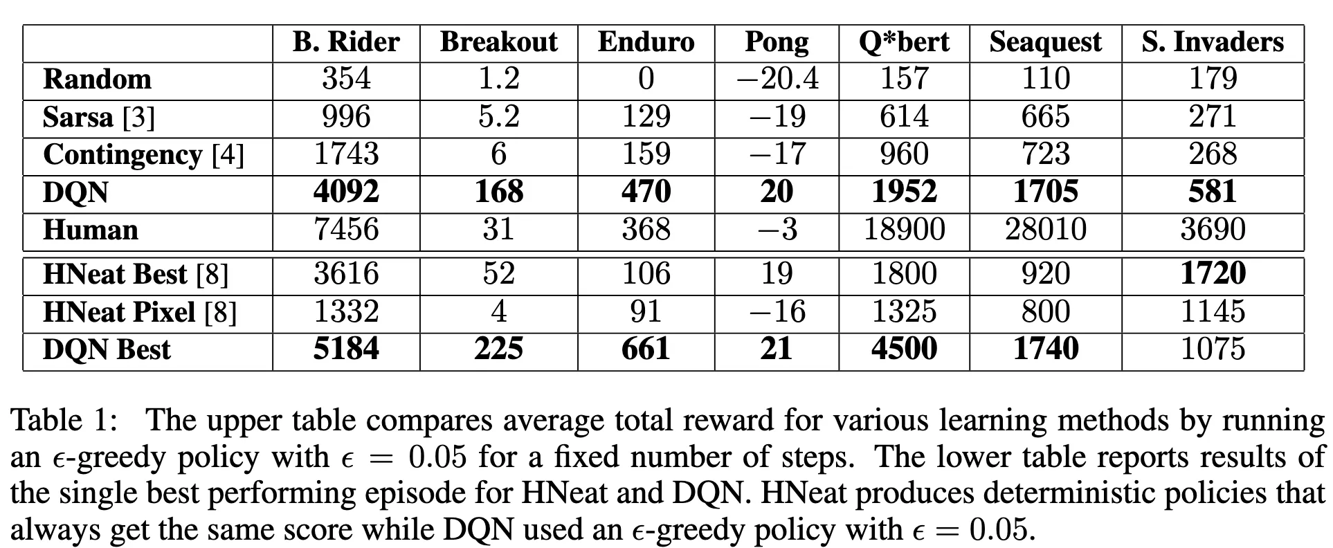
With the exact same network architecture and hyperparameters across all games, the DQN agent:

Outperformed all previous approaches on 6 out of 7 games.
Surpassed human expert-level performance on 3 games: Breakout, Enduro, and Pong.

No game-specific feature engineering. No manual tuning per game. One algorithm, seven games.

Comparison of DQN performance against other methods and human experts

Why This Paper Matters

This wasn’t just about playing video games. It was a proof of concept that a single, general-purpose learning algorithm could:

Take raw sensory input (pixels).
Learn complex, long-horizon strategies.
Master multiple tasks without task-specific modifications.

It opened the floodgates for Deep RL, leading directly to AlphaGo, OpenAI Five, and the robotic manipulation systems we see today.

Next Up

Neural Turing Machines (2014) — Can we give a neural network an external “working memory” like RAM? Coming Soon!

📚 References

Original Paper (ArXiv)